Bump Chart in Excel
 Note: The data can be as you like, it is about ranking the products or anything else, and you can place any data you want.
How to create a Bump Chart?
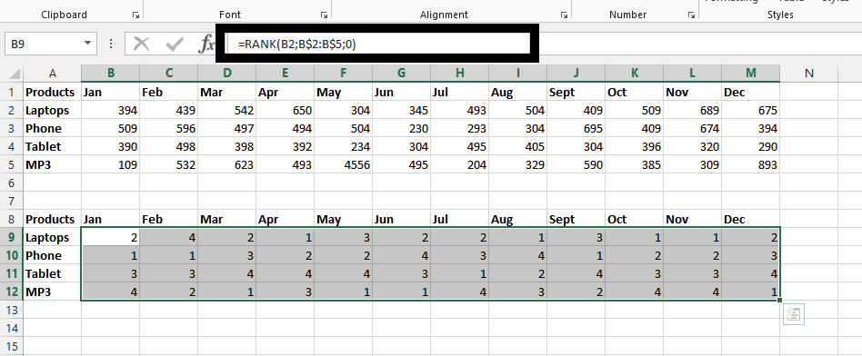
Copy the time and thing you would like to rank into a new place in the same sheet. In this case, we are going with products.

Mark the same quantities of cells with data in the data you initially has.

With the marked area, click on the formula bar, and type in =RANK(B2; all the cells in the same column, for example B$2:B$5). The full formula in my example is =RANK(B2,B$2:B$5,0). Press CTRL + Enter.

Click on any of the rank cells that is still marked.

Click on insert tab (1), and then click on Line chart (2).

Choose a line chart without marker in 2-D.

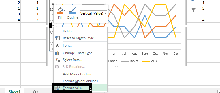
Right click on the Y axis (1), and click on format axis (2). ¨

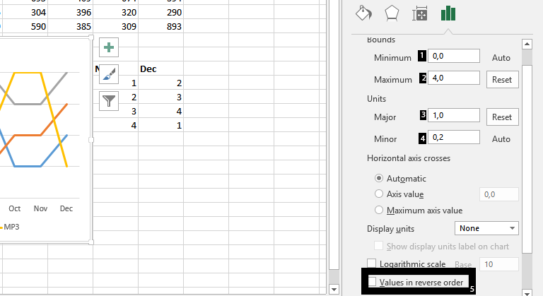
In the bound, type 0 as the minimum (1), 4 as maximum (2), 0 as minor (3), 1 as major (4), and then check values in reverse order (5).

Note: If you have 3 different things you are ranking, than four, you should set the maximum (2) to 3. You can also add an axis title if you wish.
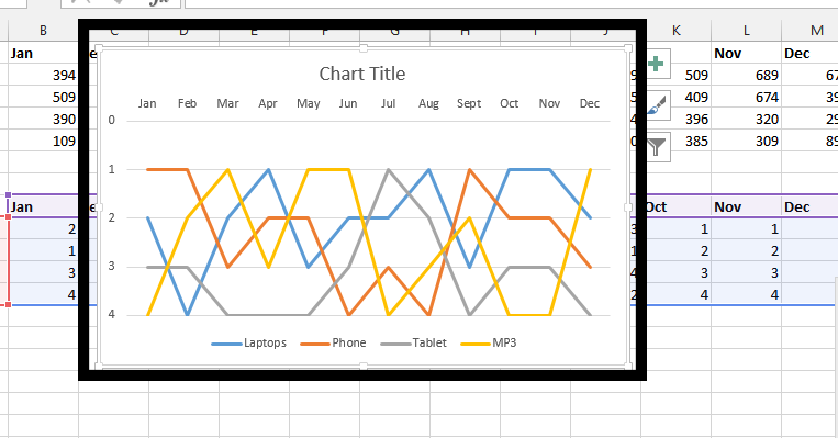
Our Bump Chart:

Template
Further reading:
Basic concepts
Getting started with Excel
Cell References


