

Excel Icon Sets
Undoubtedly visual graphics make your data look more attractive. Icons increase the readability of your text. If you’re want to make your data good-looking in Excel, you can also opt for Icon Sets. Unlike Color Scales, icon sets take a range of values and apply visual icons to represent those values.
You can display icons like traffic lights, stars, or arrows based on your values with a conditional formatting rule. For example, you can show a 0 rating star for a number less than 30, a half-filled star for a value less than 80 and greater than 30, and a 5-star Rating for values that are above 80. This conditional formatting feature is useful in representing data like using a rating system, visually showing completed jobs, representing sales numbers, etc.
What are Excel Icon Sets?
“Excel icon sets is a part of conditional formatting that helps the users to visually represent the data with arrows, shapes, check marks, flags, rating starts and other objects.”
The Icon Sets conditional formatting feature in Excel aids the users to visually represent their data with arrows, directions, shapes, checkmarks, rating stars, and other icons. It beautifies the number representation in your Excel worksheet. In Excel, you will find different types of inbuilt Icon sets options used to visualize the selected cell based on their numbers or values.
For example, you can use the star rating icon to display the ratings of any product, showing completed tasks, representing sales.
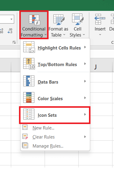
You can apply the icon sets to your data by accessing the Home menu ribbon’s conditional formatting drop-down list. All the formatting options will be displayed. Click on the icon sets option (refer to the below image).
![]()
![]()
Icon Set Options
By default there are four categories of Excel icon sets. All the icons in the list serves some purpose.
![]()
![]()
- Directional: Icons displaying colored and black arrow heads aligned at different angle to represent different directions
- Shapes: Icons representation various geometrical shapes
- Indicators: Indicating icons such as flags, cross, checkmark and exclamatory.
- Ratings: Icons displaying different rating options
If you wish to customize the color or functioning of the icons based on some criteria, you should select the More Rules? option.
Points to Remember
- Icon Sets works only if we put on accurate conditional formatting for your Excel data.
- IF you don’t apply exact formatting rules while working with Icon Sets, Microsoft excel will throw an error dialog box.
- Icon Sets are commonly used to represent the numeric data in a graphical way.
Examples
Example 1: Using Icon sets feature highlight the cell values with different object based on some criteria.
Below given is the Excel table, representing the list of household spending. Using Excel Icon sets, list down the spendings in the order of their values. Use a green circle to represent the highest figures (greater than 100), orange circles for medium values (greater than 60 and lower than 100), and red circles for lower values (below 60).
| Item | Amount |
|---|---|
| Electricity Bill | $ 150.00 |
| Water Bill | $ 60.00 |
| House Rent | $ 400.00 |
| Groceries | $ 990.00 |
| Vegetables | $ 100.00 |
| Maid | $ 150.00 |
| Children Fees | $ 800.00 |
| Car Instalment | $ 500.00 |
| Gym Membership | $ 400.00 |
The Icon Sets conditional formatting feature in Excel aids the users to visually represent their data with arrows, directions, shapes, check marks, rating stars and other different icons.
To list down the spendings with Excel icon sets in the order of their values, follow the below steps:
STEP-1 Select the range of cells
Select the cells you wish to add the icons using the Icon sets conditional formatting feature. In our case, we have to add the icons in column D. Therefore, we have selected the cells from D6 to D14.
Refer to the below image:
![]()
![]()
Step 2: Select Conditional Formatting Icon Sets
Go to the Home tab of the Excel ribbon. Apply the icon sets by selecting the Conditional Formatting (listed in Styles group) > Icon Sets
![]()
![]()
Step 3: Click on ‘More Rules’
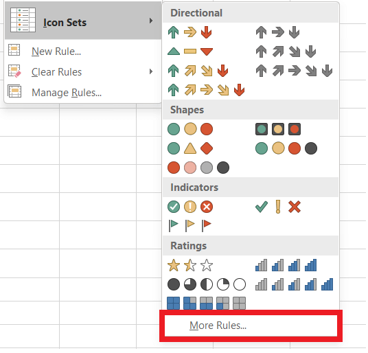
- As soon as you will click on the Icon set option. It will open a sub icon set window displaying all the inbuilt icons.
- You will find four different icon sets, including Directional (displaying colored and black arrowheads aligned in different directions), Shapes (geometric shapes), Indicators (flags, cancel, checkmark, and exclamatory), Rating (star ratings).
- Since we are asked to apply icon sets based on some criteria in our question. So we cannot go with the default option. Therefore, we will click on the ‘More Rules’ option (as shown in the below image)
![]()
![]()
Step 4: Apply the format and specific criteria
Excel will bring up ‘New Formatting Rule’ window, do the following’
- At first from the ‘Select a Rule Type:’ make sure to choose the first option i.e., ‘Format all cells based on their values’
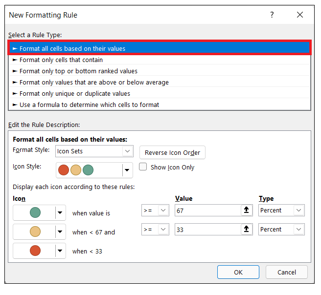

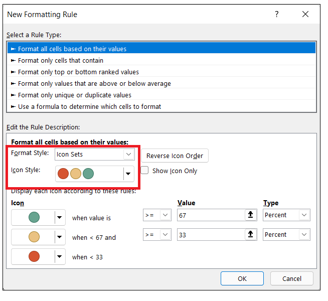
- From the ‘Edit the Rule Description:’ section, make sure to choose the Icon Sets from the Format Style dropdown.
- Choose your preferred icon option for the Icon Style dropdown.
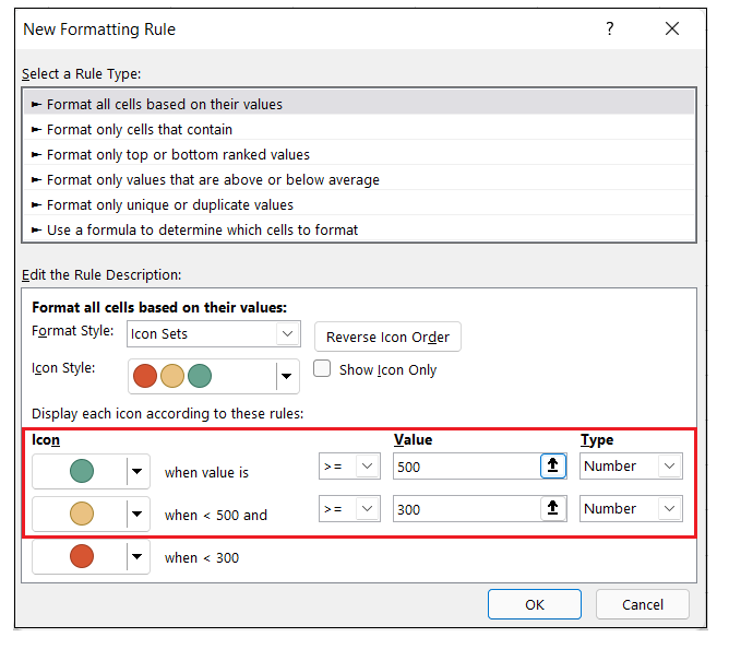
- Next, we will display each icon set according to the given criteria. In the Icon section,
- select the red icon, where the value should be greater than 100 and in the type parameter select number.
- select the orange icon, set the value to be greater than 60 and below 100 and in the type parameter select number.
- select the blue icon, and it will automatically set the last icon if the cell value is below 60.
- Click on OK
Important Tips:
- You can also change the sequence of the select icons by clicking on the Reverse Icon Order button.
- Sometimes you only require to show the icons, so you can tick the Show Icon Only check box to hide the cells’ values.
- You can assign icons based on a cell’s value instead of specifying any number or percent. Directly type the cell address in the Type parameter box.
Step-4 The icons will be applied according to the criteria
As a result, you will notice the following:
- the cells containing values greater than 500 are highlighted with red icons,
- cells containing cell values greater than 300 and smaller than 500 are highlighted with orange fill icon,
- and the cells containing values below 300 are highlighted with blue icons.
Look out at the below figure for the resulting output.
![]()
![]()
A common belief among Excel users is that Excel icon sets can only be used to format cells based on their values. But it is not all true!
With good knowledge and more effort, one can set Excel icons based on the blank and non-blank cell values in a row, as shown below.
Example 2. Apply an icon set based on blanks and non-blanks cell values
In the below example, you are given a list of data inputs for different commands. There were few errors in the command because of that it hasn’t processed any output. Using Excel Icon set add three different icons depending on whether the cells in the same row are blank or non-blank.
- Add a check mark icon if all cells in the row are filled in with values,
- Add an exclamation mark icon if some cells in the row are blank,
- Add a cross icon if all cells in a row are blank.
| C1 | C2 | C3 | C4 |
|---|---|---|---|
| 0 | 1 | 5 | 1 |
| 0 | 1 | 1 | |
| 1 | 0 | 0 | |
| 1 | 0 | 0 | |
| 0 | 1 | 0 | 1 |
Solution: To solve the above, firstly, we must find the count of the total number of blank cells in a row. For that, we will need the help of an Excel function, i.e., COUNTBLANK. To use an Excel icon set for the above criteria, execute the following steps:
Step 1: Add an Empty Column
The first step is to add an empty helper column named with ‘Icon’
![]()
![]()
In this helper column, we will count the number of blank cells present in a row.
Step 2: Count the blank cells
Next, we will use the inbuilt COUNTBLANK function of Excel. Start the function using equal to (=) function followed by COUNTBLANK. In the parameter specify the range of the row.
Your formula will become: =COUNTBLANK(B12:F12)
Refer to the below image:
![]()
![]()
Drag the formula using the ‘+’ icon to copy the formula down the cells. Don’t worry because here we have used relative range reference, so the specified range in the formula will change as per the row.
As shown below, you will have the count of blank cells in the helper column.
![]()
![]()
STEP-3 Select the range of cells
Select the cells you wish to add the icons using the Icon sets conditional formatting feature. In our case, we have selected the cells from D6 to D14.
Refer to the below image:
![]()
![]()
Step 4: Select Conditional Formatting Icon Sets
- Go to the Home tab of the Excel ribbon. Apply the icon sets by selecting the Conditional Formatting (listed in Styles group) > Icon Sets
- As soon as you will click on the Icon set option. It will open a sub icon set window displaying all the inbuilt icons.
- Since we are asked to apply icon sets based on some criteria in our question. So we cannot go with the default option. Therefore, we will click on the ‘More Rules’ option (as shown in the below image)
Step 4: Apply the format and specific criteria
Excel will bring up ‘New Formatting Rule’ window, do the following:
- At first from the ‘Select a Rule Type:’ make sure to choose the first option i.e., ‘Format all cells based on their values’
- Makesure to select the Icon sets and click the Reverse Icon Order button to change the sequence of icons.
- Tick the checkbox of ‘Show Icon Only’ to hide the values and display only the icons.
- From the Icon style, choose the Checkmark, exclamatory and cross icon set
- Choose the cross icon, set it values >=4 and in the type parameter select number.
- For the exclamation mark icon, set the value >=1 and in the type parameter select number.
Refer to the below image:
![]()
![]()
Step 5: Excel will add the icon sets according to the criteria
As a result, you will notice the checkmark icon if all the cells in the row are filled with data, an exclamatory icon if some cells are blank values and cross icon if all the cells in a row are blank.
Look out at the below figure for the resulting output.
![]()
![]()


