

Excel IFERROR() function
The IFERROR() is a logical function of Excel. It is a special function designed to catch and handle errors in formulas and calculations. Sometime while working with Excel formulas, there occurs some unexpected errors because of the improper cell value that we have used. In such cases IFERROR function allows us to replace those error messages with any other different values.
To be more specific, IFERROR checks the Excel formula, and if the formula triggers an error, the function returns another value (blank, custom text, number value, boolean) that you specify; else, if the formula doesn’t evaluate any error, it simply returns the output of the formula.
This function works on 9 formula errors generated by Excel wherever the user use any improper value or data type, such as – #N/A, #NUM!, #VALUE!, #REF!, #NAME?, #DIV/0!, or #NULL! Error.
Syntax
Parameters
Value (required): This parameter represents the first value that is evaluated to see if there occurs an error.
Value_if_error (optional): This parameter replaces the error value by this value if there is an error in the cell.
Examples
Example 1: In the below case, we have divided Data A by Data B and have displayed two outputs, one using IFERROR and one without using the IFERROR function.
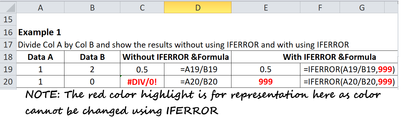
As you can see in the above example, on dividing the data value 1 by 0, Excel has thrown an error, i.e. ‘#DIV/0!’. So using IFERROR, we can give values we want unlike here where we have replaced the error with numeric data i.e, 999. You can also enter text, special symbols or some logical values which can let the user know that there is some problem with the data.
Example 2: Divide Data A by Data B and display the output without using IFERROR function and with using IFERROR function.
You can also provide customized text messages to indicate the user that there is some problem with the data.
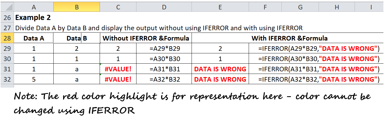
As you can see in the above example, on dividing 1 by a, we get an error (as we cannot divide a number with alphabet), without using IFERROR we get #VALUE! i.e. an error. So using IFERROR, we can give values we want unlike here we have replaced the error with a customized message i.e, “DATA IS WRONG”.
Now whenever the IFERROR finds an error it will show the same text message. You can also enter number, special symbols or some logical values which can let the user know that there is some problem with the data.
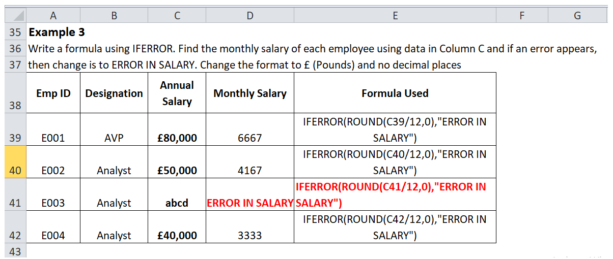
Example 3: Write an Excel formula in the below data table using IFERROR to find the monthly salary of each employee using data in Column C and if there occurs an error, replace the error message with ‘ERROR IN SALARY’. Change the format to £ (Pounds) and no decimal places (use the Round Function to avoid decimal).
| Emp ID | Designation | Annual Salary | Monthly Salary |
|---|---|---|---|
| E001 | AVP | Ł80,000 | |
| E002 | Analyst | Ł50,000 | |
| E003 | Analyst | abcd | |
| E004 | Analyst | Ł40,000 |
In the above question, we will use a combination of IFERROR and Round function. Where IFERROR function will help catch and handle errors in formulas, and if an error appears, then change it to ERROR IN SALARY. In contrast, the ROUND function will round all the calculations (if there is no error). We know salary figures are always in number, but for E003, the salary is ‘abcd’ which is not a valid number. Therefore, it will throw an error in this case, and we will catch and handle the error using the IFERROR function. Refer to the below image for the solution to the above question.
That’s it! Now, you can freely use the Excel IFERROR function to trap and manage errors the way you want.
Things to remember while working with Excel IFERROR function
- The IFERROR function operates well for types of Excel error (specifically 9 Excel formula errors) unlike #N/A, #NAME?, #DIV/0!, #NUM!, #NULL!, #REF!, and #VALUE!.
- The best thing about the IFERROR function is that it replaces the error messages with your customized text message, number, date or logical value as it looks more professional.
- IF you pass a blank cell in the value argument, it is treated as an empty string (”’) but not an error.
- The Excel IFERROR() function was initially introduced with Excel 2007 and since then it is available in all its subsequent versions such Excel 2010, 2013, 2016 and even the latest Office 365.
- To locate the error in Excel 2003 and in all its earlier versions, you can use the combination of ISERROR function with IF function. It will also work in the same way as IFERROR.
IFERROR vs. IF ISERROR
Now, as we have already discovered about the IFERROR function, its usage, syntax, parameters, implementation, you may question why some Excel users are still inclined towards using the ISERROR function (with a combination of IF). Also, you may wonder about the difference between the IFERROR function and ISERROR function in EXcel, as both sounds the same.
In the following table, we briefly discussed regarding these two major uncertainties:
| S.NO | IFERROR | ISERROR |
|---|---|---|
| 1. | The Microsoft Excel IFERROR is a special function designed to catch and cope errors in formulas and calculations. | The Microsoft ISERROR FUNCTION checks for different types of formula errors unlike, #VALUE!, #REF!, #DIV/0!, #NUM!, #NAME? and #NULL. |
| 2. | =IFERROR (Value, [Value_if_error]) | =ISERROR(value) |
| 3. | The IFFERRPR function also takes #N/A into consideration. | The ISERR function does not include the #N/A error into consideration |
| 4. | The IFERROR function was introduced with Excel 2007 and since then it is available in all its subsequent versions such Excel 2010, 2013, 2016 and even the latest Office 365. | To locate the error in Excel 2003 and in all its earlier versions, the users used the combination of ISERROR function with IF function. Therefore many Excel users still are used to of using ISERROR rather than IFERROR function. |
| 5. | It is the easiest way to trap and handle the errors. | The combination of ISERROR and IF function can also be used to catch and manage the error. It’s just a complex method to achieve the output. |
Best practices for using IFERROR in Excel
By now, we have understood the logic behind the IFERROR function and perceive that it is the easiest way to trap and manage errors in Microsoft Excel. It easily replaces the error values with blank cells, numeric data or custom text messages. However, that does not imply you should cover every Excel formula with the IFERROR function, and therefore the following suggestions may help you hold the balance.
- Don’t apply the error function without any reason. If you are sure there won’t be any error don’t use it because smaller the formula smarter is the code.
- Cover the lowest possible part of any formula in IFERROR function.
- IFERROR is not only the one way to handle errors as there are some other Excel functions as well using which you can handle only specific errors with a smaller scope:
- To trap #N/A errors use IFNA or IF ISNA function.
- To trap all errors except for #N/A use the ISERR function.


