Excel MAX() Function

MS Excel is one of the most popular spreadsheet programs with the highest numbers of supported functions. MAX() is one of the built-in Excel functions and is easy to use. The MAX function is categorized under the statistical functions on the ribbon.

This article discusses the essential method of using the Excel MAX() function with syntax and examples.

What is the MAX Function in Excel?

The MAX function is a built-in Excel function categorized as a Statistical Function. It is typically used to retrieve the maximum or largest value from a supplied set of data/ array. This function can be entered as a worksheet function; as a part of the formula within a specific cell in a worksheet.

In financial analysis, the MAX function can be used to find the highest salary of the employee, the highest score, the highest time taken, the highest expenses or revenue amount, etc.

The MAX function is supported in all versions of Excel, such as Office 365, Excel 2019, Excel 2016, Excel 2013, etc.

Syntax

The following is the syntax of MAX function in Excel:

Here, the numbers can be represented by numeric values, arrays, named range, a reference to a specific cell, or a range including the numbers.

Arguments or Parameters

Excel MAX function contains at least one compulsory argument, while the other arguments are optional.

• Compulsory Argument: number1 is a required argument and must be defined using a number, named range, array, or a reference to any number.
• Optional Argument(s): number2 and other subsequent arguments are optional. They can be defined as the same as the compulsory argument.

In Excel 2003, we can only provide up to 30 number arguments to the MAX function. However, in Excel 2007 and later, we can provide up to 255 arguments.

If an argument is given to the function as a reference to a cell, or an array of cells, the MAX function will ignore blank cells and text or logical values contained in the defined cell range. However, logical values and text representations of numbers that are passed directly to the function will be included in the calculation.

Returns

The MAX function returns the highest/largest value in numerical form from a set of data.

How to use MAX Function in Excel?

The MAX function is an easy-to-use function in Excel. It can be used as an ordinary worksheet function. This means we can apply the MAX function as a part of a formula in a cell(s) within the worksheet.

To use a MAX function as a formula in its simplest form, we can enter it directly with some random numbers in the list of arguments within a cell. For example:

In this simple example, the MAX function returns the number 3 as it is the largest one amongst given arguments. However, we usually deal with values in cells or ranges while using the MAX function in Excel. The below steps help us to apply the MAX function to find the highest value in a selected range of data:

• We must select a cell to store the highest value and enter ‘=MAX(‘ without colons.
• Next, we need to select a range of numbers or cells by a mouse.
• We must enter the closing parenthesis ‘)’ without colons.
• Lastly, we must press the Enter key.

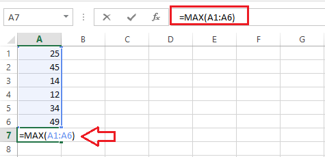
In the following sheet, we apply the MAX function in a cell A7 to find the largest value in the range A1 to A6:

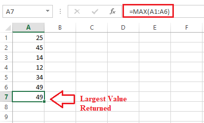
In the above example, the MAX function returns the following value as a result:

Let us now understand the working of MAX function by some other examples:

Excel MAX Function Examples

Below we discuss some typical uses of the Excel MAX function with examples:

Example 1: Finding the Max Value in a Group

To find the largest value (numeric) in a group of some number in Excel, we can apply the MAX function to the entire group by selecting it as a range. We can select any number of rows and columns within the group range.

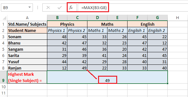
We have some students’ marks in the example below, and we need to find the highest mark.

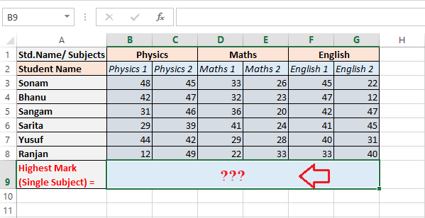
Here, we apply the MAX function to a range of cells with marks, i.e., B3 to G8. Therefore, we use =MAX(B3:G8).

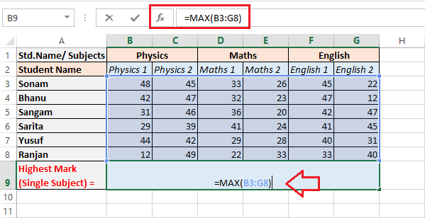
Upon pressing the Enter key, we get the maximum scored marks from the entire group of marks.

Example 2: Finding the Max Value in Non-Adjacent Cells or Ranges

Sometimes, there may be cases when we want to find the highest value for non-contiguous cells and ranges. In such a case, we must include a reference to each specific cell and/ or range. We can follow the below steps to quickly select desired non-adjacent cells or ranges and find a maximum value accordingly:

• First, we need to start typing a MAX function in a result cell. However, after typing the opening parenthesis, we must press and hold down the Ctrl button and select the desired cells and ranges within the worksheet.
• After selecting the last item, we must release the Ctrl button and type the ending parenthesis.
• Lastly, we need to press the Enter button on the keyboard.

By doing this, Excel automatically applies the corresponding syntax and provides the result accordingly.

In the example below, we have some students’ marks, and each subject’s total is also written in corresponding cells within the sheet. We need to find the highest total marks (subject-wise highest marks) obtained amongst specified subjects.

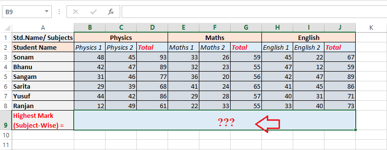
Here, we apply the MAX function to the non-adjacent cells/ range of cells with total marks per subject. When using the Ctrl button and applying the MAX function, we get a formula similar to this:

=MAX (D3:D8,G3:G8,J3:J8)

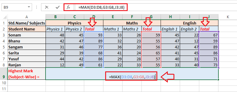
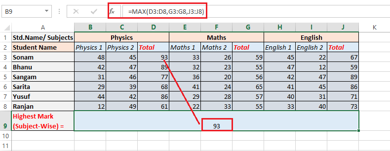
Upon pressing the Enter key, we get the maximum scored marks in any subject from the list of total marks in each subject.

Example 3: Finding the Max (Latest) Date in Excel

In Excel, the dates are treated as serial numbers. That is the reason we can use the MAX function and find the latest date with ease.

In the example below, we have some expected delivery dates for the products. To know the last date of delivery, we need to find the latest delivery date.

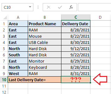
We can apply the MAX function in the same way that we use it for numbers. In our example, delivery dates are written in a range of cells from C2 to C9. Therefore, we select the result cell and apply the MAX function similar to this:

=MAX(C2:C9)

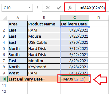
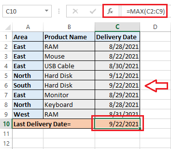
Upon pressing the Enter key, we get the latest delivery date from the list.

Example 4: Finding the Max value from Range with Cells containing Boolean Values

Sometimes, there may be cases when we want to find the highest value, but some values are written in a Boolean form. For instance, we have the following data set, and we need to find the highest score from the list in column B.

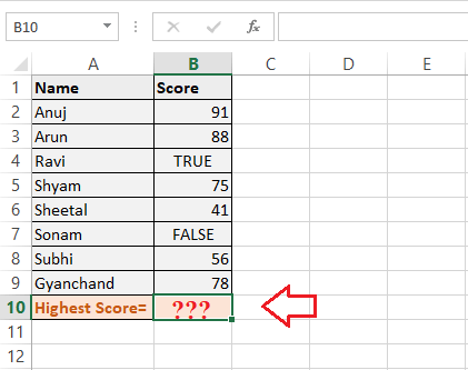
In our example data, some of the Students’ score values are Boolean. Excel MAX function does not accept or read the Boolean values and calculates the result (Max Value), ignoring particular cells.

Therefore, we can apply the MAX function in the same way that we use for numbers. In our example, students’ scores are written in a range of cells from B2 to B9. Therefore, we select the result cell (B10) and apply the MAX function similar to this:

=MAX(B2:B9)

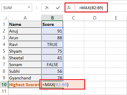
We get the highest score from the list upon pressing the Enter key, as shown in the following table.

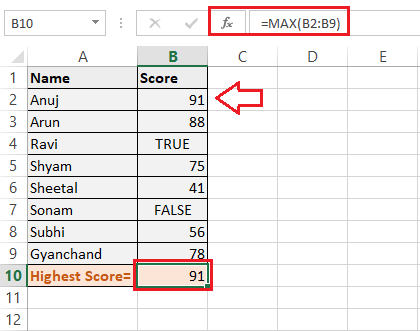
That is how we can use the MAX function in Excel.

Some Important Points to Remember

To successfully apply the MAX function in the Excel sheet, we must remember the following points:

• There is currently a maximum of 255 supported arguments that can be supplied to the MAX function in the latest version of Excel.
• If the arguments (at least one) are not supplied to the MAX function, then the MAX function returns zero (0) as output.
• If there is any non-numeric value supplied in arguments, the MAX function returns #VALUE! Error.
• Excel MAX function only accepts numbers (numerical values) and ignores the text, text values, empty cells, and the logical values TRUE and FALSE (TRUE evaluates as 1, FALSE evaluates as 0).