

Excel NPER Function
Stock analysts or financial admin often want to know how long it will take to obtain the required output when raising corporate funds. In normal banking as well, one may want to determine the total payments to repay while applying for a loan. Mostly the loans or mortgages are paid in monthly installments. However, some people prefer to pay them in quarterly or semiannually installments.
Before applying for a loan, it is good to calculate the number of required periodic payments to return the entire loan amount. Now, the question arises how one case easily find the number of periodic payments? To cater to these requirements, Excel provides an inbuilt function, the NPER function, which stands for “number of periods”.
In this tutorial, we will cover the brief insight of NPER function, including its definition, the steps to calculate the number of periods to return the loan, or the number of investments needed to reach the target amount, various examples, situations where NPER may not work in Excel and more!
What is NPER function?
The Excel NPER calculates the number of payments required based on the fixed interest rate, constant periodic payments.
The NPER function is a financial function in Excel used to return the number of periods for an investment or bank loan. There are many uses of the NPER function, such as it assists in fetching the number of payment periods for a loan, for a specified amount, the rate of interest, and the periodic payment amount. The function was introduced with Excel 2007 and since then is available in all versions including Excel 2010,Excel 2013, Excel 2016, Excel 2017 and Excel 365.
Syntax
Parameter
Rate (required)- This argument represents the rate of interest per period.
pmt (required)- This argument represents the payment made for each period.
pv (required)- This argument represents the current value, or total value of all payments now.
fv [optional]: This argument represents the future value, or a cash balance the user want after the last payment is made. Since it is an optional parameter therefore its default value is 0.
type [optional]: This argument provides the information regarding when payments are due.
- If the user provides 0 it means end of period
- If he supplies 1, it means beginning of period. Since it is an optional parameter therefore its default value is 0.
Points to Remember about NPER Function
Kindly have a look at the below given point to efficiently utilize the NPER function in your worksheets and bypass common mistakes in Excel:
- Use positive numbers for inflows (the amounts that you get) and negative numbers for outflows (the amounts that you pay).
- If the value for pv parameter is zero or omitted, in that case the fv parameter must be included.
- You can specify the rateparameter as a percentage or decimal number, for instance 23% or .23.
- Always ensure to supply the interest ratecorresponding to periods. For instance, if the loan is to be paid monthly at an annual interest rate of 26%, then use 26%/12 or 0.26/12 for the rate parameter.
Examples
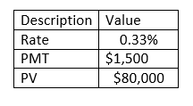
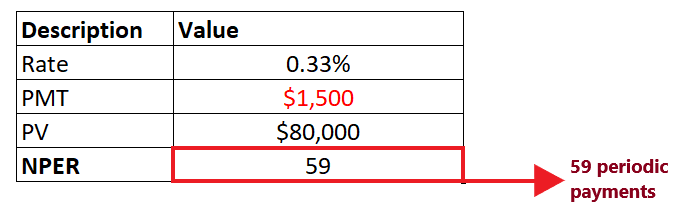
Example 1: Calculate the number of periodic payments for a loan using NPER function for the below given values.
To determine the periodic rate payment follow the below given steps:
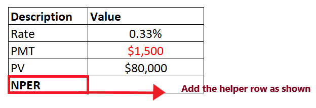
Step 1: Add helper row at the bottom of table
Put your cursor below the table and add your helper row. In this row we will type the NPER formula and will fetch the periodic payment for the given data.
Refer to the below image:
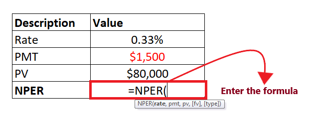
Step 2: Enter the NPER formula
Move to next cell of your helper row and start typing the formula = NPER(
It will look similar to the below image:
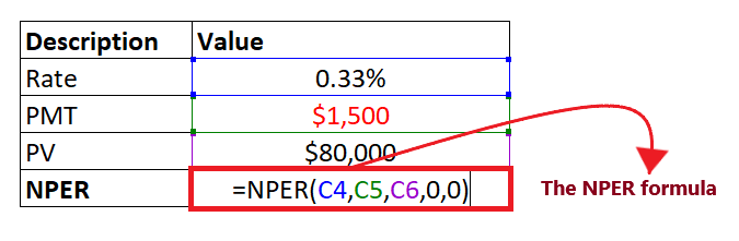
STEP 3: Add the parameter to your formula
- In the first parameter, we will specify the interest rate per period. In the above table, the rate is mentioned in cell C4. So our formula becomes: =NPER (C4,
- Next, this function will ask for the pmt This parameter represents the payment made for each period. The pmt is mentioned in cell C5. So our formula becomes: =NPER (C4, C5
- The pv parameter represents the current value, or total value of all payments. It is mentioned in cell C6. So our formula becomes: =NPER (C4, C5, C6
- The fv is an optional parameter that represents the future value, or a cash balance the user want after the last payment is made. Since it is an optional parameter therefore its default value is 0. So our formula becomes: =NPER (C4, C5, C6, 0
- This last parameter, i.e., type, is optional. In this, we specify the information regarding when payments are due. Since we want the payment for the end of the period, so we will specify 0. So our formula becomes: =NPER (C4, C5, C6, 0, 0)
The overall formula will look similar to the below image:
STEP 4: NPER will return the output
Press the enter button as soon as you are done typing the formula. Excel will return the output for your NPER formula. As shown below it will return 59 as an output of your periodic payment.
Therefore, we can conclude that ABC will have to make 59 monthly payments of $1,500.
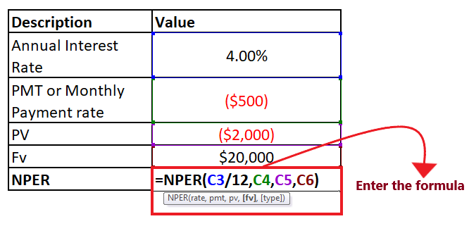
Example 2: Suppose you want to invest an amount of $2,000 at an annual interest rate of 4% and make an extra contribution of $100 at the end of every month. Your aim is to reach at $20,000. Calculate the number of monthly investments including the given future value (fv) in the NPER formula.
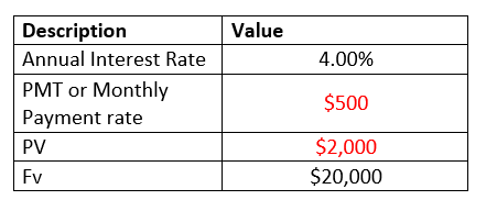
NOTE: In the above table the inputs pmt and pv are negative numbers (represented by red text color) because they denote an outflow.
To determine the number of monthly investments follow the below given steps:
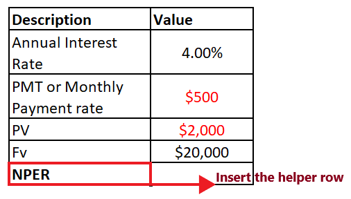
Step 1: Add helper row at the bottom of table
Put your cursor below the table and type the heading of your helper row i.e., “NPER”. In this row we will type the NPER formula and will fetch the periodic payment for the given data.
Refer to the below image:
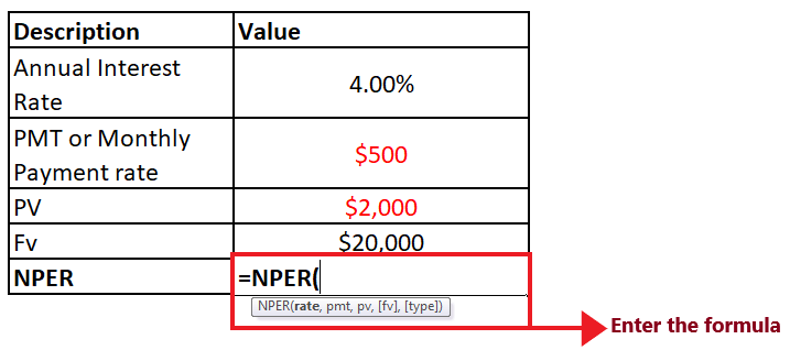
Step 2: Enter the NPER formula
Move to next cell of your helper row and start typing the formula = NPER(
It will look similar to the below image:
STEP 3: Add the parameter to your formula
- In the first parameter, we will specify the interest rate per period. Since we have to return the periods in months, we will divide the rate argument by 12 (number of periods per year). So our formula becomes =NPER (C3/12,
- Next, we will specify the pmt The negative PMT signifies an outflow payment made for each period. The pmt is mentioned in cell C4. So our formula becomes: =NPER (C3/12, C4
- The pv parameter represents the current value, or total value of all payments. It is mentioned in cell C5. So our formula becomes: =NPER (C3/12, C4, C5
- The future value (fv) is already mentioned in the above table. So our formula becomes: =NPER (C3/12, C4, C5, 0
- This last parameter (type) is omitted since the payments are due at the end of the period.
The overall formula will look similar to the below image:
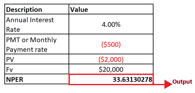
STEP 4: NPER will return the output
Press the enter button as soon as you are done typing the formula. Excel will return the output for your NPER formula. As shown below it will return 33.6 as an output of your periodic payment.
Therefore, we can conclude that it will take ABC 33.6 monthly investments to reach the target amount.
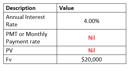
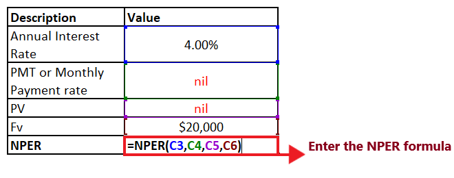
Example 3: In the below table, few of the arguments are non-numeric. Let’s see what happens if you specify non-numeric arguments in NPER formula.
To fetch the NPER output for the above table follow the below given steps:
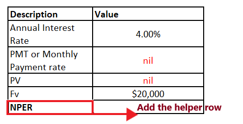
Step 1: Add helper row at the bottom of table
Put your cursor below the table and add your helper row. In this row we will type the NPER formula and will fetch the periodic payment for the given data.
Refer to the below image:
STEP 2: Add the formula and its parameters
- Move to next cell of your helper row and start typing the formula = NPER(
- Add all the five NPER parameters and you will receive the below formula = =NPER(C3,C4,C5,C6)
NOTE: We have omitted the type parameter as we have assumed the payments are due at the end of the period.
STEP 3: NPER will return a #VALUE! error
Press the enter button as soon as you are done typing the formula. Excel will return the output for your NPER formula. As shown below it will throw the #VALUE! error.
Refer to the below image:
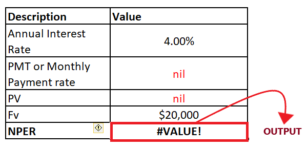
This error occurs if any of the arguments specified in your NPER formula is non-numeric. To fix this error in Excel, always ensure that all the parameters are numeric and all the specified numbers are not formatted as text.
Excel NPER function not working
Sometimes while working with the NPER function, there are possibilities you might run into an error or a wrong result, and it mostly occurs because of one of the following reasons:
- #NUM! error
This error occurs if the given fv argument is never obtained with the specified rate (interest rate) and pmt (payment) parameters. Suppose you want to obtain a valid NPER result, attempt to raise a periodic interest rate and/or a payment amount.
- #VALUE! error
This error occurs if any of the arguments specified in your NPER formula is non-numeric. To fix this error in Excel, always ensure that all the parameters are numeric and all the specified numbers are not formatted as text.
- The output of NPER function is a negative number
This problem occurs in the NPER formula when you have used positive numbers to represent the outflow payments. For example, when you calculate the payment periods for a loan, provide the pv (loan value) parameter as a positive number and the pmt argument as a negative number.


