What’s New in Excel 2010?
New Features in Excel 2010
Sparklines
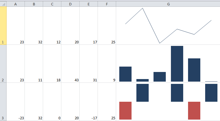
Sparklines are small charts which you can insert in a cell and link to data in other cells. You can insert sparklines of 3 types depending upon your data: line, column and win/loss. You can find these sparklines by going to the Insert menu ribbon bar.

Step 1. Open Excel 2010 and save the file as new.xlsx. Enter data as shown below.

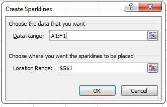
Step 2. Click cell G1 and go to Insert –> Sparklines –> Line and you will get a new window. In the Data Range: textbox, enter A1:F1 and click OK.
Step 3. Similarly, insert column sparkline in G2 and win/loss sparkline in G3. Increase the width and height of the rows so that you are able to see the sparklines clearly.
Screenshot
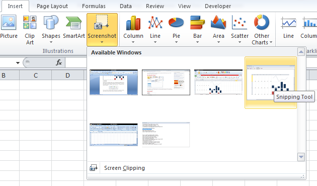
Using the new screenshot feature you can quickly grab screenshots of any open window and embed those screenshots in your documents. You can find the screenshot feature by going to Insert (main menu) –> Screenshot (in the illustrations group).

Once you click the Screenshot option, you will see screenshots of all the open windows. You just need to click the screenshot you want to insert.
Improved Ribbon
Excel 2010 allows you to customize the ribbon the way you want. You can create custom tabs and groups and even change the order or name of the built-in tabs and groups.
Go to File –> Options and you will get a new window. Select Customize Ribbon from the left hand side.
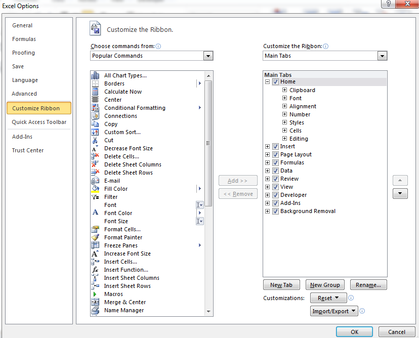
You can add a new tab by clicking New Tab button. You just need to select the commands from the left and click the Add button to add the required commands to your new tab. You can rename an existing tab or group by selecting the particular tab or group from the right and clicking the Rename button. You can add a new group to the existing tab by clicking New Group button. You can change the order of tabs or groups using the up and down arrows at the right. Here, I have created a new tab named MyTab with 4 commands Center, Insert Function, Line and Spelling. From the window, you could see that the new tab is added after the Insert tab.
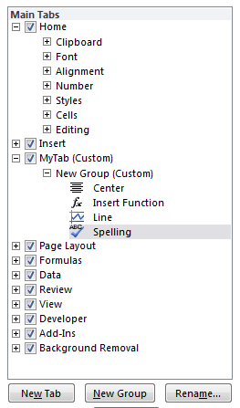
You could see this new tab in the Excel file as well.

Slicer
Slicer allows you to slice and dice pivot tables so that you can visualize your data more effectively. You can find the new Slicer feature by going to Insert (main menu) –> Slicer (in the Filter group).

Step 1. To create a pivot table, enter data as in the following image.
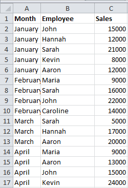
Step 2. Select cells A1:B17 and go to Insert (main menu) — Pivot table (from the Tables group). Select Existing Worksheet option and click any cell where you want to insert your pivot table. Click OK.
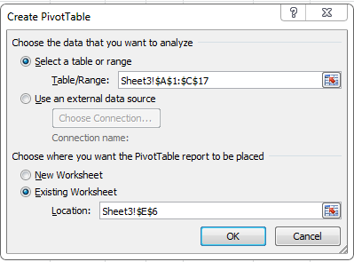
Now you will get a new window to create your pivot table. Make it as in the following image by checking the items at the top and dragging and dropping items as required.
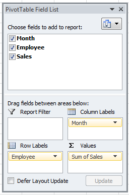
Now you are ready with your pivot table.
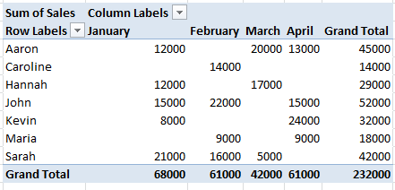
Step 3. Click somewhere inside the pivot table and go to Insert (main menu) –> Slicer (in the Filter group). You will get a window like this:
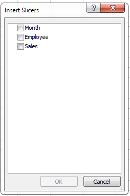
You can click the options you want to analyze in detail. If you check Month, you will get a window like this:
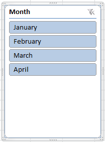
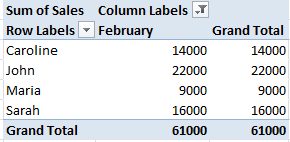
If you click a month, say February, you will get the details for that particular month.
There are many more subtle UI enhancements, features and improvements in Excel 2010.


